45 how to add labels to a scatter plot in excel

Add labels to scatter graph - Excel 2007 | MrExcel Message Board I don't simply want the numerical value or 'series 1' for every point - but something like 'Firm A' , 'Firm B' . 'Firm N' The only way I can find of doing this thus far is to create a new 'series' for EVERY row in the table - and then manually edit the points to all look the same and display the label! - Very long winded and time consuming! How to add axis label to chart in Excel? - ExtendOffice Click to select the chart that you want to insert axis label. 2. Then click the Charts Elements button located the upper-right corner of the chart. In the expanded menu, check Axis Titles option, see screenshot: 3. And both the horizontal and vertical axis text boxes have been added to the chart, then click each of the axis text boxes and enter ...

How to create a scatter plot and customize data labels in Excel During Consulting Projects you will want to use a scatter plot to show potential options. Customizing data labels is not easy so today I will show you how th...

How to add labels to a scatter plot in excel

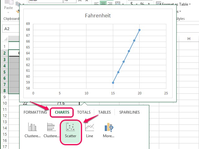
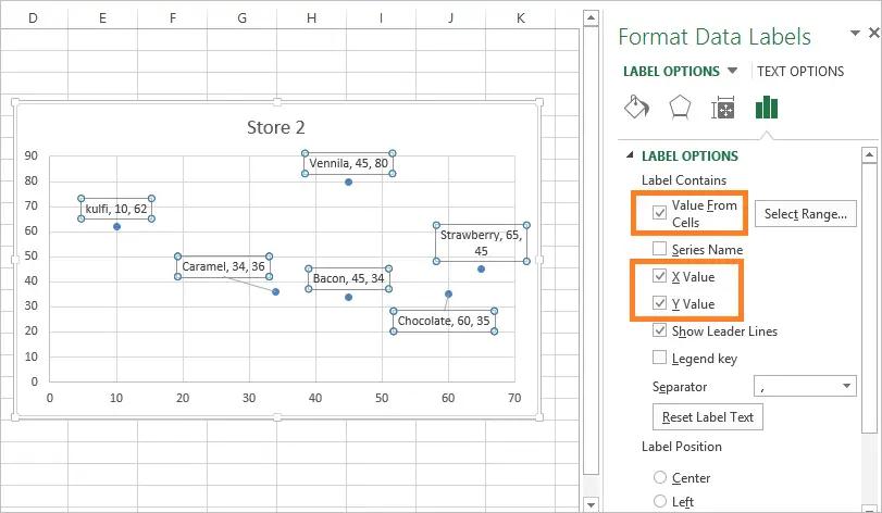
How to use a macro to add labels to data points in an xy scatter chart ... Press ALT+Q to return to Excel. Switch to the chart sheet. In Excel 2003 and in earlier versions of Excel, point to Macro on the Tools menu, and then click Macros. Click AttachLabelsToPoints, and then click Run to run the macro. In Excel 2007, click the Developer tab, click Macro in the Code group, select AttachLabelsToPoints, and then click Run. excel - How to label scatterplot points by name? - Stack Overflow This is what you want to do in a scatter plot: right click on your data point. select "Format Data Labels" (note you may have to add data labels first) put a check mark in "Values from Cells". click on "select range" and select your range of labels you want on the points. Add Custom Labels to x-y Scatter plot in Excel Step 1: Select the Data, INSERT -> Recommended Charts -> Scatter chart (3 rd chart will be scatter chart) Let the plotted scatter chart be. Step 2: Click the + symbol and add data labels by clicking it as shown below. Step 3: Now we need to add the flavor names to the label. Now right click on the label and click format data labels.

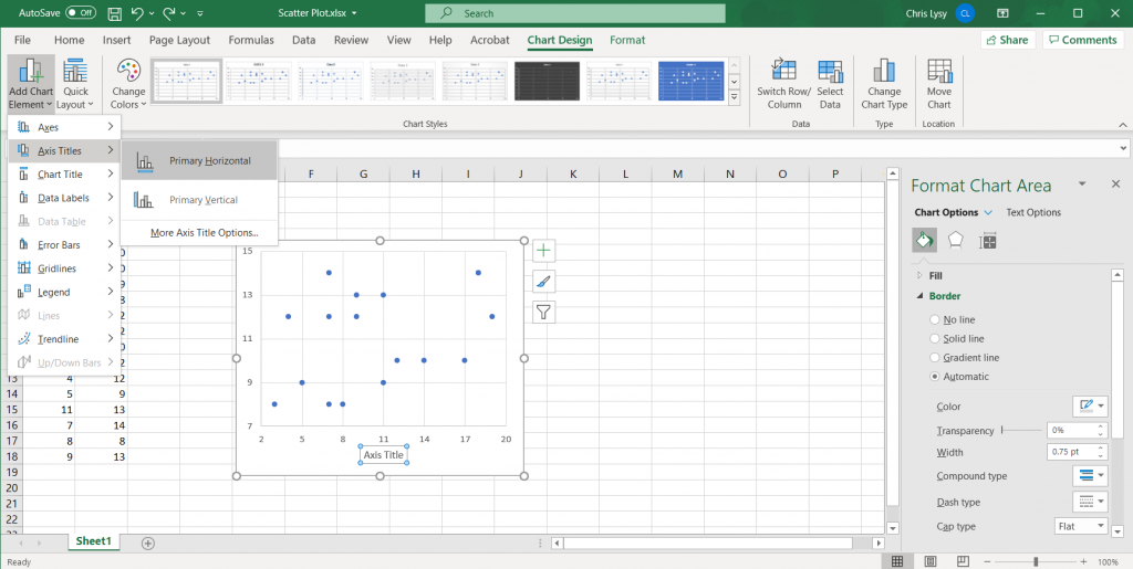
How to add labels to a scatter plot in excel. Use text as horizontal labels in Excel scatter plot Edit each data label individually, type a = character and click the cell that has the corresponding text. This process can be automated with the free XY Chart Labeler add-in. Excel 2013 and newer has the option to include "Value from cells" in the data label dialog. Format the data labels to your preferences and hide the original x axis labels. How To Add Axis Labels In Excel [Step-By-Step Tutorial] First off, you have to click the chart and click the plus (+) icon on the upper-right side. Then, check the tickbox for 'Axis Titles'. If you would only like to add a title/label for one axis (horizontal or vertical), click the right arrow beside 'Axis Titles' and select which axis you would like to add a title/label. Editing the Axis Titles Labels for data points in scatter plot in Excel - Microsoft Community Answer HansV MVP MVP Replied on January 19, 2020 Excel 2016 for Mac does not have this capability (but Microsoft is working on it - see Allow for personalised data labels in XY scatter plots) See Set custom data labels in a chart for a VBA macro to do this. --- Kind regards, HansV Report abuse How to Make a Scatter Plot in Excel | GoSkills Step 1: Organize your data. Ensure that your data is in the correct format. Since scatter graphs are meant to show how two numeric values are related to each other, they should both be displayed in two separate columns. The first column will usually be plotted on the X-axis and the second column on the Y-axis.

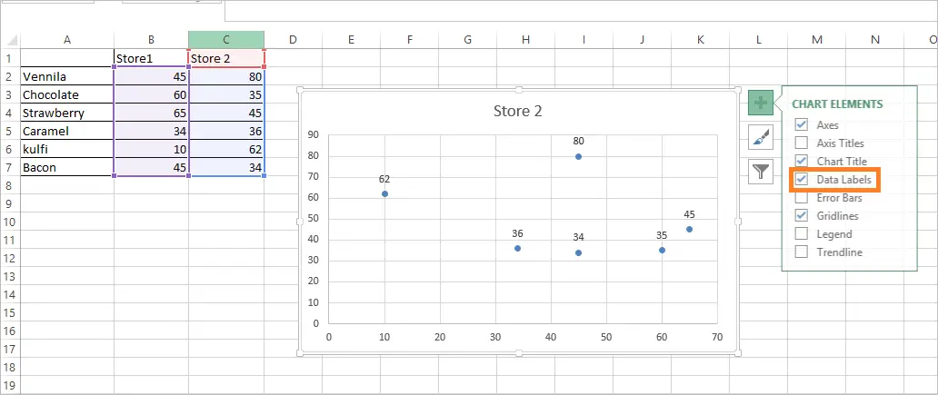
How to add conditional colouring to Scatterplots in Excel Step 3: Edit the colours. To edit the colours, select the chart -> Format -> Select Series A from the drop down on top left. In the format pane, select the fill and border colours for the marker. Repeat these steps for Series B and Series C. Here is our final scatterplot. Improve your X Y Scatter Chart with custom data labels Press with right mouse button on on a chart dot and press with left mouse button on on "Add Data Labels" Press with right mouse button on on any dot again and press with left mouse button on "Format Data Labels" A new window appears to the right, deselect X and Y Value. Enable "Value from cells" Select cell range D3:D11 How to find, highlight and label a data point in Excel scatter plot To let your users know which exactly data point is highlighted in your scatter chart, you can add a label to it. Here's how: Click on the highlighted data point to select it. Click the Chart Elements button. Select the Data Labels box and choose where to position the label. How to add labels to the mosaic plot - Microsoft Excel 2016 This is the third, and last part of the tip How to create a mosaic plot in Excel (the second part is How to create a step Area chart for the mosaic plot). ... To add the labels for the mosaic pieces, do the following: 1. Create a new data range to calculate the positions of each label: For every mosaic piece from the prepared data:

How can I add data labels from a third column to a scatterplot? Under Labels, click Data Labels, and then in the upper part of the list, click the data label type that you want. Under Labels, click Data Labels, and then in the lower part of the list, click where you want the data label to appear. Depending on the chart type, some options may not be available. How to Find, Highlight, and Label a Data Point in Excel Scatter Plot? By default, the data labels are the y-coordinates. Step 3: Right-click on any of the data labels. A drop-down appears. Click on the Format Data Labels… option. Step 4: Format Data Labels dialogue box appears. Under the Label Options, check the box Value from Cells . Step 5: Data Label Range dialogue-box appears. How to Create a Scatterplot with Multiple Series in Excel Step 3: Create the Scatterplot. Next, highlight every value in column B. Then, hold Ctrl and highlight every cell in the range E1:H17. Along the top ribbon, click the Insert tab and then click Insert Scatter (X, Y) within the Charts group to produce the following scatterplot: The (X, Y) coordinates for each group are shown, with each group ... How to Quickly Add Data to an Excel Scatter Chart Set the minimum bound to -0.2 and the maximum to 0.2. Scroll down in the task pane to Number and reduces the decimal places to 2. Close the task pane. To finish formatting this chart, we'll add appropriate labels. To add a title to the new axis, click in the chart area and select the green plus sign.

Add Custom Labels to x-y Scatter plot in Excel - DataScience Made Simple

How to Add Labels to Scatterplot Points in Excel - Statology Step 3: Add Labels to Points. Next, click anywhere on the chart until a green plus (+) sign appears in the top right corner. Then click Data Labels, then click More Options…. In the Format Data Labels window that appears on the right of the screen, uncheck the box next to Y Value and check the box next to Value From Cells.

How to Make an XY Graph on Excel | Techwalla.com

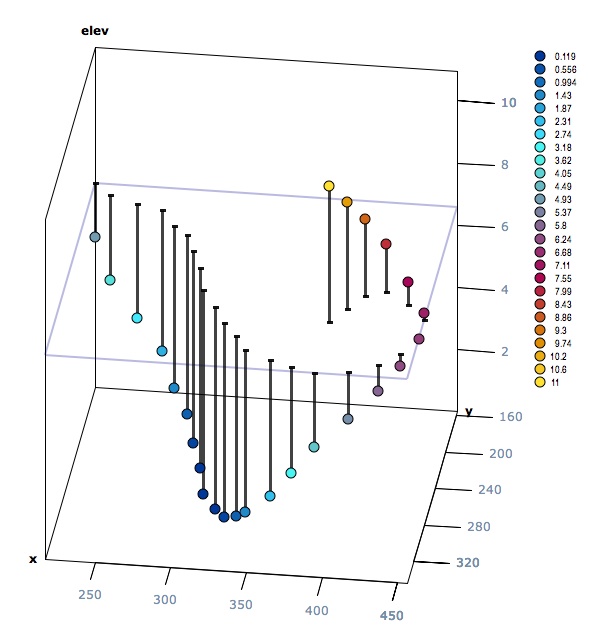
How to make a scatter plot in Excel - Ablebits 3D scatter plot in Excel; Scatter graph and correlation; Customizing scatter plot. Adjust the axis scale to reduce white space; Add Excel scatter plot labels; Add a trendline; Swap X and Y data series; Scatter plot in Excel. A scatter plot (also called an XY graph, or scatter diagram) is a two-dimensional chart that shows the relationship ...

How to Make Scatter Plots in Microsoft Excel 2007

How to Make a Scatter Plot in Excel and Present Your Data Add Labels to Scatter Plot Excel Data Points. You can label the data points in the X and Y chart in Microsoft Excel by following these steps: Click on any blank space of the chart and then select the Chart Elements (looks like a plus icon). Then select the Data Labels and click on the black arrow to open More Options.

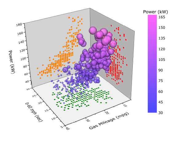
3D Graphs in Origin

Add or remove data labels in a chart - support.microsoft.com Add data labels to a chart Click the data series or chart. To label one data point, after clicking the series, click that data point. In the upper right corner, next to the chart, click Add Chart Element > Data Labels. To change the location, click the arrow, and choose an option.

How To Make A Scatter Plot In Excel

How can i add data labels in the scatter graph? [SOLVED] Re: How can i add data labels in the scatter graph? If you want to link the data labels to the cells, then select the chart and run this code once: Please Login or Register to view this content. Then when you change the cells, the data labels should update automatically. Register To Reply. 06-07-2016, 10:24 AM #6.

excel - Add line to Scatter Plot - Stack Overflow

How to display text labels in the X-axis of scatter chart in Excel? Display text labels in X-axis of scatter chart Actually, there is no way that can display text labels in the X-axis of scatter chart in Excel, but we can create a line chart and make it look like a scatter chart. 1. Select the data you use, and click Insert > Insert Line & Area Chart > Line with Markers to select a line chart. See screenshot: 2.

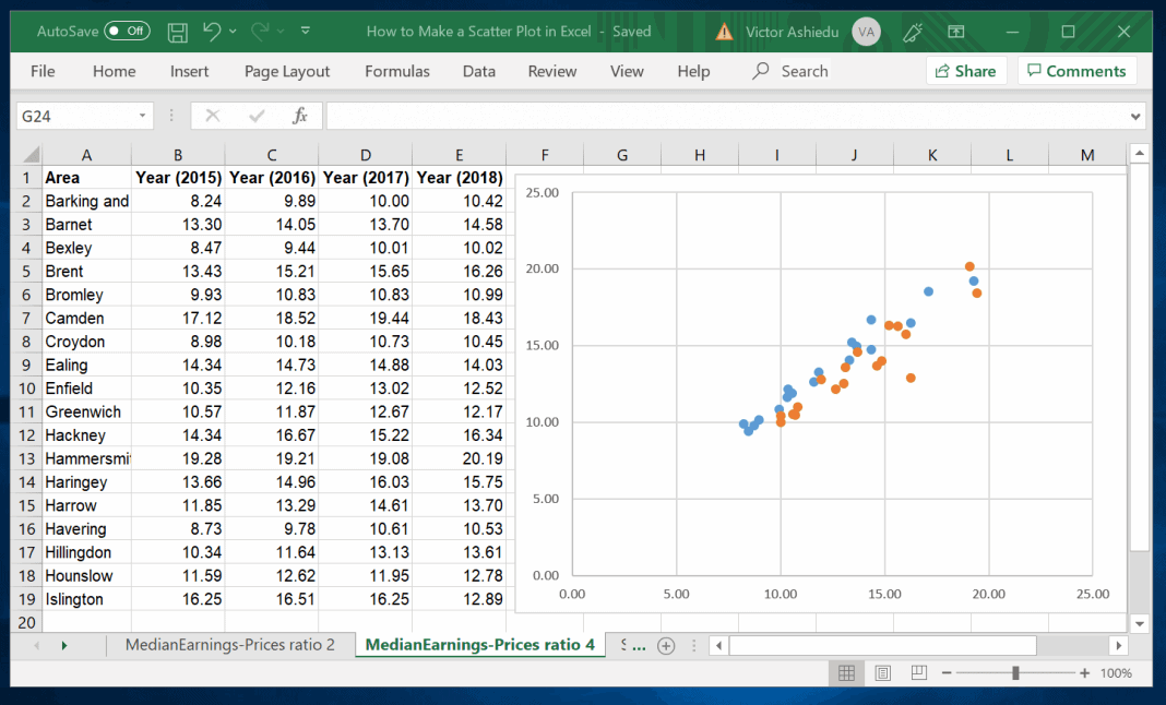
How to Make a Scatter Plot in Excel | Itechguides.com

How do I get a label in a scatter plot instead of "Series 1 Point"? They are not actually labels, by the way. They show series name, point number (the X value), and the X and Y values in parentheses. Yeah, X appears twice. In order to see the location, you need to set up the chart to have one series per row of the data. Tedious by hand, though possible. Easier with VBA.

Add Custom Labels to x-y Scatter plot in Excel - DataScience Made Simple

Hover labels on scatterplot points - Excel Help Forum For a new thread (1st post), scroll to Manage Attachments, otherwise scroll down to GO ADVANCED, click, and then scroll down to MANAGE ATTACHMENTS and click again. Now follow the instructions at the top of that screen. New Notice for experts and gurus:

charts - Excel: Individual labels for data points in a group - Stack Overflow

How to Create Scatter Plot In Excel - Career Karma 2. Display the Scatter Chart. Once you have inputted the data, select the desired columns, go to the Insert tab in Excel, select the XY Scatter Chart and choose the first scatter plot option. Now you should have a scatter graph shown in your Excel file. With this done, you need to add a chart title to the scatter plot.

How to Create Scatter Plots in Excel - EvalCentral Blog

Excel 2019/365: Scatter Plot with Labels - YouTube How to add labels to the points on a scatter plot.

How to Make a Scatter Plot in Excel | Itechguides.com

Add Custom Labels to x-y Scatter plot in Excel Step 1: Select the Data, INSERT -> Recommended Charts -> Scatter chart (3 rd chart will be scatter chart) Let the plotted scatter chart be. Step 2: Click the + symbol and add data labels by clicking it as shown below. Step 3: Now we need to add the flavor names to the label. Now right click on the label and click format data labels.

3d scatter plot for MS Excel

excel - How to label scatterplot points by name? - Stack Overflow This is what you want to do in a scatter plot: right click on your data point. select "Format Data Labels" (note you may have to add data labels first) put a check mark in "Values from Cells". click on "select range" and select your range of labels you want on the points.